05:00
Week 11 Starter File
Intermediate Modeling

In the second part of the course we will leverage the following resources:
- The Tidy Modeling with R book second portion of the course book
- The Tidy Models website second portion of the course website
Link to other resources
Internal help: posit support
External help: stackoverflow
Additional materials: posit resources
While I use the book as a reference the materials provided to you are custom made and include more activities and resources.
If you understand the materials covered in this document there is no need to refer to other resources.
If you have any troubles with the materials don’t hesitate to contact me or check the above resources.
Class Objectives
- Going beyond the basic by making predictions and assessing multiple models.
Load packages
This is a critical task:
Every time you open a new R session you will need to load the packages.
Failing to do so will incur in the most common errors among beginners (e.g., ” could not find function ‘x’ ” or “object ‘y’ not found”).
So please always remember to load your packages by running the
libraryfunction for each package you will use in that specific session 🤝
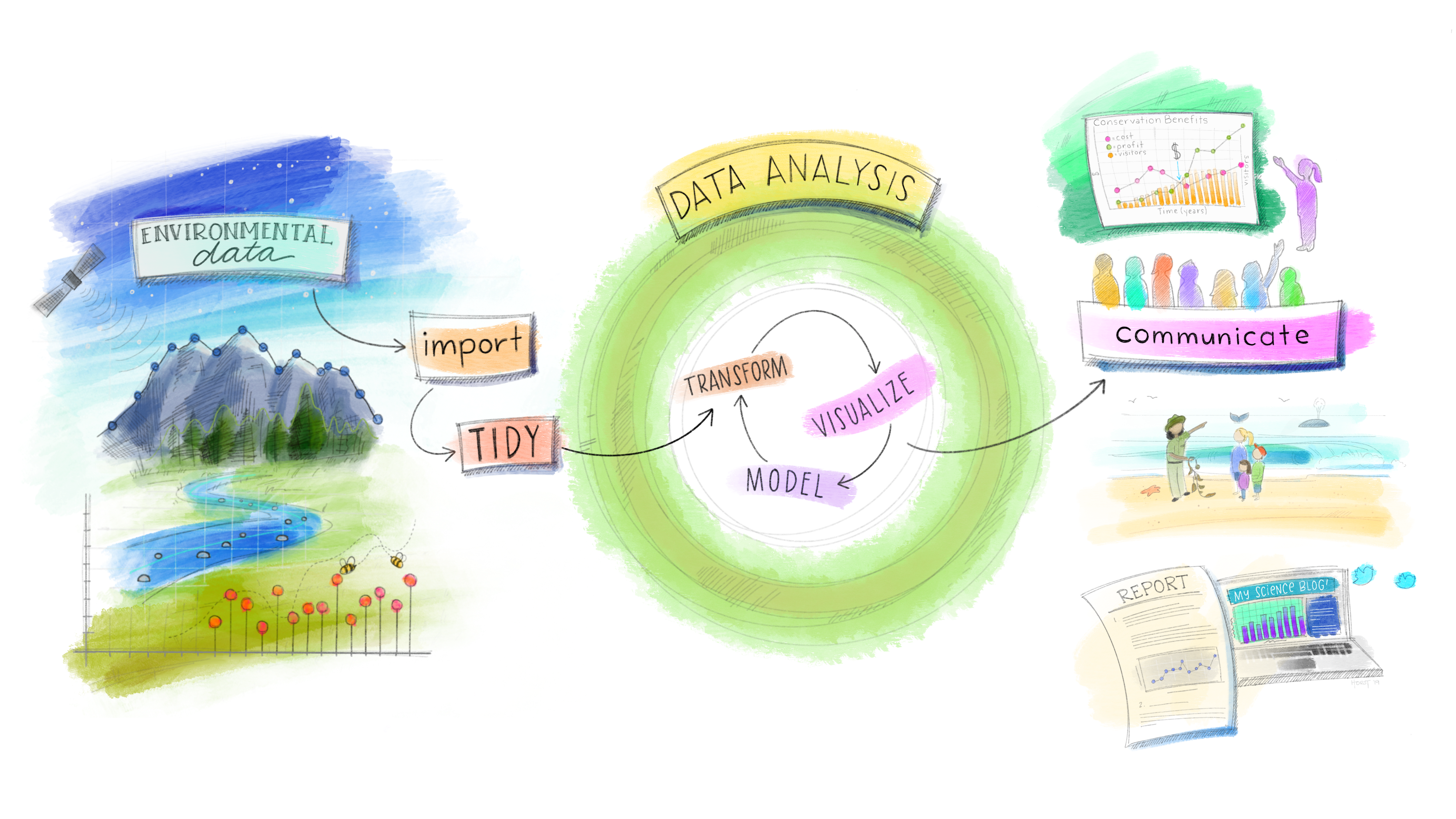
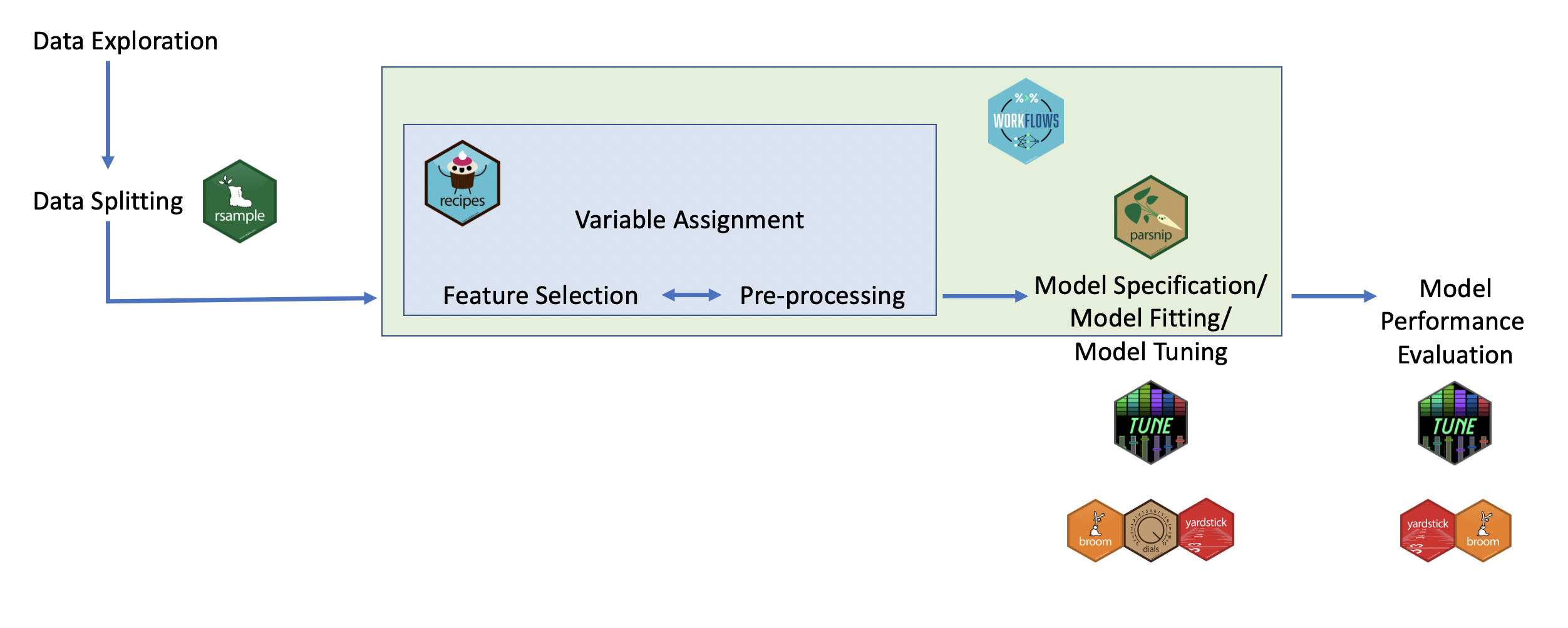
The tidymodels Ecosystem in action
Some additional useful/required steps
So far we have covered the basic of modeling and we have learned how to create recipes, define models and embed them into workflows. However, from experience there is a set of other things that are important and need to be taken care in addition of what we learned in the model basic part.
Data cleaning and generalizable manipulations
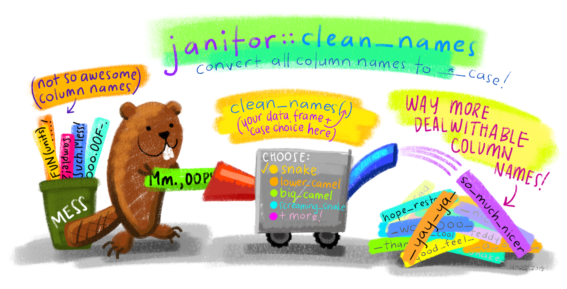
In the previous weeks we have made some repetitive transformations (e.g., log Sale_Price) and encountered constant issues with our dataset (e.g., upper and lower case columns names). It is now time to clean the data and make model independent useful manipulations before moving back to modeling
Caution
I have removed the variables that are highly correlated with the variables we will use in the models below. Remember with mutate we have created those variables from existing variables in our dataset. If you don’t remove them they will bias your results due to multicollinearity (high correlation with the original ones).
Check variables correlations
After we have made the necessary changes to the original dataset, we should investigate variables correlation. This is extremely useful when you have many numerical columns in our dataset and we want to quickly see if there are relationships between them. THe focus should be on the dependent variables at first.
A positive (blue) or negative (red) correlation between two variables indicates the direction of the relationship between them:
Positive Correlation: A positive correlation indicates that the two variables move in the same direction. When one variable increases, the other variable also tends to increase, and similarly, when one decreases, the other tends to decrease. This relationship reflects a direct association between the variables, where changes in one variable are mirrored by changes in the other in the same direction, either upwards or downwards. The correlation is considered positive whenever its value is greater than 0. A perfect positive correlation, with a coefficient of +1, means that the two variables move in the same direction in a perfectly linear manner.
Negative Correlation: A negative correlation indicates that the two variables move in the opposite directions. When one variable increases, the other variable tends to decrease, and viceversa. This inverse relationship means that changes in one variable are associated with opposite changes in the other, highlighting an indirect association between them. The correlation is considered negative whenever its value is smaller than 0. A perfect negative correlation, with a coefficient of -1, means that the two variables move in opposite directions in a perfectly linear manner.
Interpreting Correlations:
Magnitude of the Coefficient: The closer the correlation coefficient is to +1 or -1, the stronger the linear relationship between the variables. A correlation of 0 indicates no linear relationship.
Significance of the Correlation: It’s also important to assess the statistical significance of the correlation. A correlation coefficient might indicate a positive or negative relationship, but statistical tests (like a significance test for correlation) can determine if the observed correlation is not likely due to random chance. These tests are beyond the scope of the class but you need to be aware that it is good practice to perform them.
Causation: It’s crucial to remember that correlation does not imply causation. Even if two variables have a strong positive or negative correlation, it does not mean that one variable causes the changes in the other. Other variables, known as confounding variables, could influence the relationship, or it could be coincidental. Regression will help us in understanding how the dependent variable changes with an independent variable, holding other factors constant. This is particularly useful for controlling for potential confounders and examining the specific impact of one variable on another.
Chart interpretation: By looking at our correlation plot we can tell that all variables selected have a positive correlation with
price_log. It appears that the stronger correlation is withtotal_sfwhich means that larger houses tend to sell for higher prices (when one increases the other does the same). The only variables that are slightly negatively correlated arebedroom_abvandyear_built, which is interesting. Try to interpret more variables in the chart on your own.
Activity 1: Computing, visualizing and interpreting correlation. Write the code to complete the tasks below - 8 minutes
[Write code just below each instruction; finally use MS Teams R - Forum channel for help on the in class activities/homework or if you have other questions]
Create a “correlation_matrix2” that includes price_log, kitchen_abv_gr, tot_rms_abv_grd, fireplaces, garage_cars, garage_area, wood_deck_sf, open_porch_sf, longitude, latitude.
Create a plot that visually shows the correlation between the variables computed with the above matrix.
Interpret the correlation chart. Here are some prompts for you: What variable/s have positive correlation with sale_price? Pick one and interpret what it means. What about variables with negative correlation? Pick one and interpret what it means. Anything surprising?
Data Splitting and Cross-validation
Now that we have checked the correlation and made some changes to our ames dataset, we can move back to modeling. So far we have run our models on the entire ames dataset. However, by doing so we have no data left to evaluate and assess our model performance on unseen data. Here are the two commonly used methods to preserve data for assessing models performance:
Data Splitting
Cross-validation
While a simple train-test split is quicker and easier, especially for exploratory analysis or when computational resources are limited, cross-validation provides a more thorough and unbiased evaluation of the model’s performance. The choice between these methods depends on the specific needs of your project, including the size of the dataset, the computational complexity of the models, and the level of accuracy required in the performance estimation. Due to time constrains we will only learn train-test split but remember that cross-validation might be what is required to assess models in some of your future data analytics projects.
Data Splitting
When it comes to data modeling (and model evaluation), one of the most adopted method is to split the data into a training set and a test set from the beginning. Here’s how this simple method can be implemented and its implications:
- Benefits of Train-Test Split:
- Simplicity and Speed: It’s straightforward to understand, implement and computationally less intensive than other methods.
- Direct Evaluation: Provides a clear, direct way to assess how the model performs on unseen data.
- Something to consider:
- Potential Data Wastage: Splitting the dataset reduces the amount of data available for training the model, which might be a concern for smaller datasets.
- Risk of Bias: If the split is not representative, it can introduce bias in the evaluation, making the model appear to perform better or worse than it actually does. Less robust than other methods.
Activity 2: Data Splitting. - 5 minutes
[Write code just below each instruction; finally use MS Teams R - Forum channel for help on the in class activities/homework or if you have other questions]
Set a random seed to reproduce the data splitting.
Define a data split with a 80/20 proportion, call the split as “ames_split2”. Compare the size of the ames_split2 with the one of the ames_split.
Create a ames_train2 and a ames_test2 object.
Example: Making prediction and evaluating different models’ prediction performance with data splitting
It is time to use a practical example to see how we can define different models and how we can assess them. We will explore the predictions’ outcome among linear regression, lasso regression and decision tree. We will do that using different recipes customized to the restrictions/needs of the different models. We will use recipe 1 and 2 with the multiple linear regression models and recipe 3 and 4 with our decision tree model.
Setting up the recipes
Important
In real life you should prep and bake recipe 1 and 2 to verify that the preprocessing steps applied lead to the desired outcomes.
Specifying the models
We will specify two regression models and a decision tree-based model using parsnip. Please see below a brief overview of the models we will use to create and evaluate predictions:
- Linear Regression
When to Use: Ideal for predicting continuous outcomes when the relationship between independent variables and the dependent variable is linear.
Example: Predicting house prices based on attributes like size (square footage), number of bedrooms, and age of the house.
- Lasso Regression
When to Use: Similar to Ridge regression but can shrink some coefficients to zero, effectively performing variable selection (L1 regularization). Useful for models with a large number of predictors, where you want to identify a simpler model with fewer predictors.
Example: Selecting the most impactful factors affecting the energy efficiency of buildings from a large set of potential features.
- Decision Tree
When to Use: Good for classification and regression with a dataset that includes non-linear relationships. Decision trees are interpretable and can handle both numerical and categorical data.
Example: Predicting customer churn based on a variety of customer attributes such as usage patterns, service complaints, and demographic information.
Fitting the models using workflows
Next, we fit the models to the ames_train dataset because we want to assess their predictions performance on the ames_test. This is accomplished by embedding the model specifications within workflows that also incorporate our preprocessing recipes.
Regression models workflows
Tree-based models workflows
Important
Don’t worry we will learn how to interpret and visualize these models in the next class.
Model Comparison and Evaluation
Before learning how to interpret all the models results, we will learn to assess their performance (there is no point in interpreting them if they perform poorly or are “bad” models). This involves making predictions on our test set, and evaluating the models using metrics suited for regression tasks, such as RMSE (Root Mean Squared Error) or MAE (Mean Absolute Error) or R² (Coefficient of Determination).
Making predictions and Evaluating Model Performance with Data Splitting
Regression models predictions
Important
Can we compute the difference between the sale_price and the predicted price? What about the sum of the errors? [hint: use mutate and summarize]
Tree-based models predictions
Caution
If you guys noticed when we run predictions using the linear regression model with recipe2 (recipe2_predictions_reg) we got a warning. The warning indicated some rank-deficiency fit. This is usually due to:
the presence of highly correlated predictors (multicollinearity). Multicollinearity indicates that we have redundant information from some highly correlated predictors, making it difficult to distinguish their individual effects on the dependent variable.
the presence of too many predictors in our model. If the model includes too many predictor variables relative to the number of observations, it can lead to a situation where the predictors cannot be uniquely identified. Meaning that there isn’t enough independent information in the data to estimate the model’s parameters (the coefficients of the predictor variables) with precision.
Possible solutions are check for multicollinearity and using correlation matrix to identify and then remove highly correlated predictors. Or reduce the number of predictors by performing Principal Components Analysis (PCA). PCA is beyond the scope of this class but regularization methods (e.g., Ridge or Lasso regression) are designed to handle multicollinearity (Ridge in particular), high number of predictors (Lasso in particular) and overfitting. For this reason we don’t get a warning when we run the lasso model using recipe2.
In conclusion, while the linear regression model with recipe2 runs (and produce just a warning), we should not attempt to interpret the results because they can misleading and lead to bad decisions. For illustrative scope we will keep that model in but we know that in real life we will have to make changes to what predictors are included in it.
Creating Model Metrics to Assess Model Prediction Performance
While seeing the predictions next to the actual house values can already provide some insights on the goodness of the model. In regression analysis, model performance is evaluated using specific metrics that quantify the model’s accuracy and ability to generalize. Three fundamental metrics are Root Mean Squared Error (RMSE) , Mean Absolute Error (MAE), and R-squared (R²):
- Root Mean Squared Error (RMSE):
- What It Measures: RMSE calculates the square root of the average squared differences between the predicted and actual values. It represents the standard deviation of the residuals (prediction errors).
- Interpretation: A lower RMSE value indicates better model performance, with 0 being the ideal score. It quantifies how much, on average, the model’s predictions deviate from the actual values.
- Something to consider: RMSE is sensitive to outliers. High RMSE values may suggest the presence of large errors in some predictions, highlighting potential model weaknesses.
- Mean Absolute Error (MAE):
- What It Measures: MAE quantifies the average magnitude of the errors between the predicted values and the actual values, focusing solely on the size of errors without considering their direction. It reflects the average distance between predicted and actual values across all predictions.
- Interpretation: MAE values range from 0 to infinity, with lower values indicating better model performance. A MAE of 0 means the model perfectly predicts the target variable, although such a scenario is extremely rare in practice.
- Something to consider: MAE provides a straightforward and easily interpretable measure of model prediction accuracy. It’s particularly useful because it’s robust to outliers, making it a reliable metric when dealing with real-world data that may contain anomalies. MAE helps in understanding the typical error magnitude the model might have in its predictions, offering clear insights into the model’s performance.
- R-squared (R²):
- What It Measures: R², also known as the coefficient of determination, quantifies the proportion of the variance in the dependent variable that is predictable from the independent variables. It provides a measure of how well observed outcomes are replicated by the model.
- Interpretation: R² values range from 0 to 1, where higher values indicate better model fit. An R² of 1 suggests the model perfectly predicts the target variable.
- Something to consider: R² offers an insight into the goodness of fit of the model. However, it does not indicate if the model is the appropriate one for your data, nor does it reflect on the accuracy of the predictions.
Regression models performance metrics
Decision tree models performance metrics
Identify the best model using models’ metrics
Decide which model to proceed with should be based on these metrics, considering RMSE \[lower values better\], MAE \[lower values better\] and R² \[higher values better\]. Sometimes the best model is the one that gives the best compromise among those metrics. They are not always in agreement. Moreover, keep in mind that the choice of model might also depend on other factors such as:
Interpretability and complexity of the model.
Computational resources and time available.
The specific requirements of your application or project.
Let’s check all the models metrics to establish the best model keeping in mind the above bullet points.
Combine All Metrics and Compare
Based on the results above we can conclude that:
The linear regression model with recipe 2 has the best MAE. However, that model is troublesome (remember the warning) and it would be very hard to interpret.
The decision tree model with recipe 4 is the best model metrics wise, it has the second lowest MAE and the best RMSE and RSQ. Decision tree are usually easy to interpret but using all the predictors might be challenging and unnecessary (more parsimonious models that lead to similar results are preferred).
Unfortunately, the more parsimonious/simpler models (e.g., recipe 1 and 3 models and lasso with recipe 2) are not close to the best models in terms of performance. So, it seems that none of the above models is truly optimal for our needs. However, we have some indications of the direction for our next model: include more than 2/3 predictors (not performing well enough) but not all predictors (too complex and harder to interpret). We will use the activities below to try to improve the current model performance.
Activity 3: Comparing and evaluating models new models - 30 minutes
[Write code just below each instruction; finally use MS Teams R - Forum channel for help on the in class activities/homework or if you have other questions]
Build a new recipe that use only numeric variables with strong positive correlation with sales price (log version) [hint: remember to create correlation matrices]. Make sure all the independent variables are standardized. Include also overall_cond and neighborhood as dummy variables. Call this recipe as “recipe_3a”.
Define a new ridge regression model using parsnip. Name the model as “linear_mod_ridge”. Make sure to use the right arguments to perform ridge regression.
Create 5 new workflows: 1) linear regression model with recipe_3a (recipe3a_workflow_reg); 2) lasso regression model with recipe_3a (recipe3a_workflow_lasso); 3) ridge regression model with recipe1 (recipe1_workflow_ridge); 4) ridge regression model with recipe2 (recipe2_workflow_ridge); 5) ridge regression model with recipe_3a. (recipe3_workflow_ridge).
Make predictions using the 5 new workflows. Call the prediction as recipe3a_predictions_reg, recipe3a_predictions_lasso, recipe1_predictions_ridge, recipe2_predictions_ridge, recipe3a_predictions_ridge.
Calculate for each one of the above RMSE, MAE and R-squared. Use similar naming convention used in the example above. Make sure to put the metrics in a new tibble. Make sure the tibble also contains the previous models results. Compare the results with the old ones. Which one is the best model in making predictions?